
Ever since I moved to Minneapolis and started working at Exosite, I’ve been using R almost daily to get to the bottom of ops mysteries. Sometimes it pays off and sometimes it doesn’t, but it’s always interesting.
Here’s an enigma I recently had the pleasure to rub some R on.
Huh…
One fine day, after a release of Portals (our webapp that lets you work with data from your cloud-enabled devices), I noticed something odd in the server metrics. The 90th-percentile response time had increased by a factor of four!
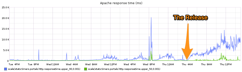
This would be alarming by itself, but here’s what made it interesting. We have two different ways of reporting the response time of our application. We have the Apache response time metric from the access logs (which is shown above), but we also have a metric generated by the PHP application itself, through statsd. A timer is initialized as soon as the PHP script starts running, and its value is reported as a timer when it’s done. And the PHP metric, for the same time period, looked like this:

This does not follow the same pattern. Sure there’s some variability, but they’re both response time: shouldn’t they follow each other more closely? And let’s look at the 90th-percentile times for Apache (blue) and PHP (red) on a common scale:
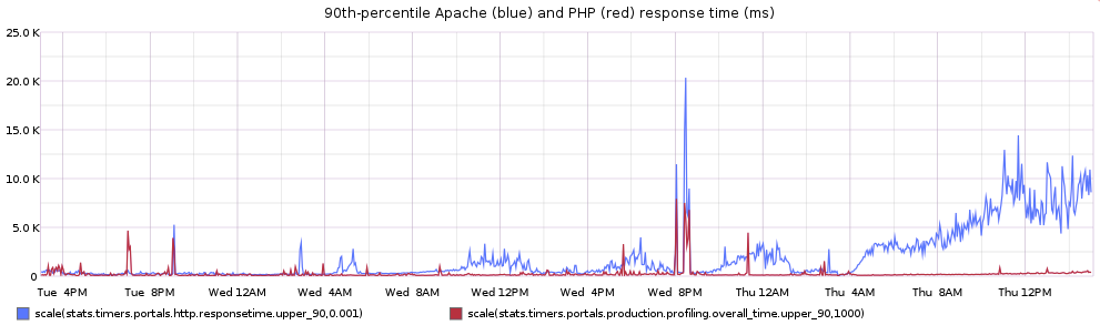
Oh whoops — I should have warned you not to be drinking water when you looked at that graph. Sorry if you ruined your keyboard. Apache’s 90th-percentile response time is way higher than PHP’s. Like way higher. What gives?
Let’s summarize what we know so far:
- 90th-percentile response times, as reported by Apache, have climbed above 5 seconds, which is much higher than normal.
- PHP response times have not experienced any such climb, so something Apache-specific is causing this behavior.
- Median values were not affected for either metric, so this issue is only affecting a particular subset of traffic.
Now it’s time to do some R.
Munging is my middle name
This disagreement between Apache response times and PHP response times is really intriguing, and might hint us toward the origin of the issue, so let’s dig into it.
The first thing to do is pull some access log entries into R. We aggregate and parse our logs with Logstash, so each entry is a JSON blob like this (irrelevant bits snipped for brevity):
{

    "@fields": {

        "agent": "Mozilla/5.0 (Windows NT 6.1) AppleWebKit/537.36 (KHTML, like Gecko) Chrome/30.0.1599.37 Safari/537.36",

        "bytes": 2660,

        "clientip": "XXX.XXX.XXX.XXX",

        "hostheader": "portals.exosite.com",

        "overall_time": 0.097,

        "request": "/manage/devices",

        "response": "200",

        "servtime": 106908

    },

    "@timestamp": "2013-08-22T14:51:32.000Z",

    "@type": "apache_access"

}
The servtime field is the Apache response time in microseconds, and the overall_time field is the PHP response time in seconds. I’ve got a script that goes and grabs a time-slice of logs from the log server and converts them to CSV format, and the result looks like this:
"@timestamp","overall_time","servtime","hostheader"

"2013-08-21T13:00:49.000Z",0.083,93408,"foo.exosite.com"

"2013-08-21T13:00:48.000Z",0.173,185900,"foo.exosite.com"

"2013-08-21T13:00:46.000Z",0.094,104675,"bar.exosite.com"

"2013-08-21T13:00:46.000Z",0.122,131222,"foo.exosite.com"

"2013-08-21T13:00:46.000Z",0.132,141991,"bar.exosite.com"

"2013-08-21T13:00:46.000Z",0.096,106194,"baz.exosite.com"

"2013-08-21T13:00:46.000Z",0.136,146550,"bar.exosite.com"

"2013-08-21T13:00:46.000Z",0.154,163942,"foo.exosite.com"

"2013-08-21T13:00:46.000Z",0.174,184448,"bar.exosite.com"
Which is perfect for slurping into R like so:
> reqdata <- read.csv("/tmp/reqdata.csv", header=TRUE, as.is=TRUE)

> # Parse the timestamps with Hadley's lubridate package

> reqdata$X.timestamp <- parse_date_time(reqdata$X.timestamp, "ymdHMs")

> # Remember, Apache response times are in microseconds, so we want to scale them to seconds

> reqdata$servtime <- reqdata$servtime / 10^6
And now we have a data frame called reqdata with a row for each log entry:
> head(reqdata)

          X.timestamp overall_time servtime          hostheader

1 2013-09-13 13:00:49        0.083 0.093408 foo.exosite.com

2 2013-09-13 13:00:48        0.173 0.185900 foo.exosite.com

3 2013-09-13 13:00:46        0.094 0.104675 bar.exosite.com

4 2013-09-13 13:00:46        0.122 0.131222 foo.exosite.com

5 2013-09-13 13:00:46        0.132 0.141991 bar.exosite.com

6 2013-09-13 13:00:46        0.096 0.106194 baz.exosite.com
The plot coagulates
Now that we have a nicely formatted data frame (we would also have accepted a pretty flower from your sweetie), we can use ggplot to check it out.
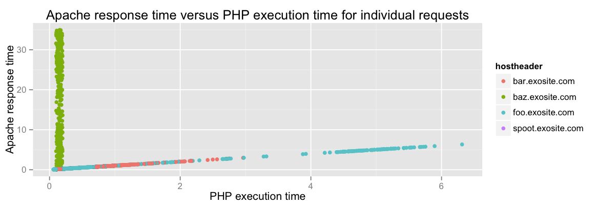
To get a handle on the Apache/PHP response time dichotomy, let’s plot one versus the other:
> p <- ggplot(reqdata, aes(overall_time, servtime))

> p + geom_point() +

    # A blue line showing the 1-to-1 relationship that we'd naïvely expect

    geom_abline(intercept=0, slope=1, color=I('blue')) +
ggtitle('Apache response time versus PHP execution time for individual requests') +
ylab('Apache response time') +
xlab('PHP execution time')

So we can see here that most of the requests are doing what we expect: getting sent to PHP as soon as they come in, and getting sent back to the client as soon as they’re done. That’s what the blue line indicates: it’s a line of slope 1.
But then we’ve got this big near-vertical chunk of weird. Those are requests where PHP finished quickly (consistently under 200 milliseconds) but Apache took much longer to serve the request (up to 35 seconds). What is Apache doing for so long? Why can’t it just serve content like it’s supposed to?
We can get a big clue if we color the points by Host header (the domain requested by the browser):
p + geom_point(color=hostheader)
Now we’re getting somewhere! Look at all that green. That means that this issue is limited to a particular domain: baz.exosite.com.
The home stretch
Okay, so now we know:
- Requests for baz.exosite.com are sitting around in Apache for up to 35 seconds before being delivered
- Our PHP executes very quickly for this domain — it’s only Apache that’s sucking up the time
Given that this traffic is limited to a particular domain, I’m getting the suspicion that there are other homogenous things about it. And we can confirm this (pretend I’d pulled in the user-agent and client IP address from the logs with my initial import):
> Filter down our dataset to just the baz.exosite.com requests

> baz <- subset(reqdata,hostheader=='baz.exosite.com')

> unique(baz$useragent)

[1] "Mozilla/5.0 (Windows NT 6.1) AppleWebKit/537.36 (KHTML, like Gecko) Chrome/30.0.1599.37 Safari/537.36"
There’s only one browser hitting this domain. Is there only one IP too? (These IPs have been changed to protect the irrelevant)
> unique(baz$clientip)

[1] "257.8.55.154"   "257.28.192.38"  "257.81.101.4"   "257.119.178.94"
Now let’s skip to the most neato part. I plotted Apache response time versus time over the course of 2 hours, faceted by client IP address. It looks like this:
ggplot(baz, aes(X.timestamp, servtime)) + geom_point(aes(color=clientip)) + facet_grid(clientip ~ .)
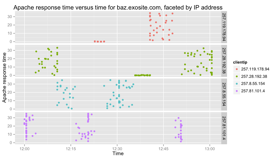
So what are we looking at? Here’s what I think.
Only one person, let’s call him François, uses this domain. François has a Portal with several auto-refreshing widgets on it. Also, François is on a train, and he’s using a wireless access point to browse the internet.
François has his Portal open in a tab that he’s forgotten about. It’s dutifully refreshing his widgets every few seconds, but as the train moves, François’s access point keeps switching towers. It starts getting a weak signal, it switches towers, François’s IP address therefore changes, and repeat.
PHP only logs how long it took to execute a script on the server, but Apache logs how long it takes for the client to acknowledge receipt of the final TCP segment in the response. Since François is on an ever-changing series of unreliable networks, he’s dropping packets left and right. Therefore, Apache is logging response times all over the map.
Alas
Alas, this information is useless. Sometimes that happens: sometimes you dig and dig and learn and learn and prepare your beautiful data, only to find at the last minute that it was all for naught.
But at least you learned something.
