
Wouldn’t you like to live in a world where your monitoring systems only alerted when things were actually broken? And wouldn’t it be great if, in that world, your alerts would always fire if things were broken?
Well so would everybody else. But we don’t live in that world. When we choose a threshold for alerting, we usually have to make a tradeoff between the chance of getting a false positive (an alert that fires when nothing is wrong) and the chance of getting a false negative (an alert that doesn’t fire when something is wrong).
Take the load average on an app server for example: if it’s above 100, then your service is probably broken. But there’s still a chance that the waiting processes aren’t blocking your mission-critical code paths. If you page somebody on this threshold, there’s always a chance that you’ll be waking that person up in the middle of the night for no good reason. However, if you raise the threshold to 200 to get rid of such spurious alerts, you’re making it more likely that a pathologically high load average will go unnoticed.
When presented with this tradeoff, the path of least resistance is to say “Let’s just keep the threshold lower. We’d rather get woken up when there’s nothing broken than sleep through a real problem.” And I can sympathize with that attitude. Undetected outages are embarrassing and harmful to your reputation. Surely it’s preferable to deal with a few late-night fire drills.
It’s a trap.
In the long run, false positives can — and will often — hurt you more than false negatives. Let’s learn about the base rate fallacy.
The base rate fallacy
Suppose you have a service that works fine most of the time, but breaks occasionally. It’s not trivial to determine whether the service is working, but you can write a probe that’ll detect its state correctly 99% of the time:
- If the service is working, there’s a 1% chance that your probe will say it’s broken
- If the service is broken, there’s a 1% chance that your probe will say it’s working
Naïvely, you might expect this probe to be a decent check of the service’s health. If it goes off, you’ve got a pretty good chance that the service is broken, right?
No. Bad. Wrong. This is what logicians and statisticians call the “base rate fallacy.” Your expectation hinges on the assumption that the service is only working half the time. In reality, if the service is any good, it works almost all the time. Let’s say the service is functional 99.9% of the time. If we assume the service just fails randomly the other 0.1% of the time, we can calculate the true-positive rate:
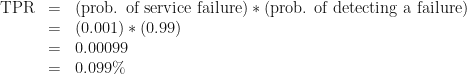
That is to say, about 1 in 1000 of all tests will run during a failure and detect that failure correctly. We can also calculate the false-positive rate:
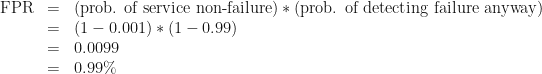
So almost 1 test in 100 will run when the service is not broken, but will report that it’s broken anyway.
You should already be feeling anxious.
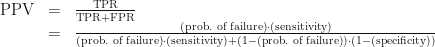
With these numbers, we can calculate what the medical field calls the probe’s positive predictive value: the probability that, if a given test produces a positive result, it’s a true positive. For our purposes this is the probability that, if we just got paged, something’s actually broken.

Bad news. There’s no hand-waving here. If you get alerted by this probe, there’s only a 9.1% chance that something’s actually wrong.
Car alarms and smoke alarms
When you hear a car alarm going off, do you run to the window and start looking for car thieves? Do you call 9-1-1? Do you even notice car alarms anymore?
Car alarms have a very low positive predictive value. They go off for so many spurious reasons: glitchy electronics, drunk people leaning on the hood, accidental pressing of the panic button. And as a result of this low PPV, car alarms are much less useful as theft deterrents than they could be.
Now think about smoke alarms. People trust smoke alarms. When a smoke alarm goes off in a school or an office building, everybody stops what they’re doing and walks outside in an orderly fashion. Why? Because when smoke alarms go off (and there’s no drill scheduled), it frequently means there’s actual smoke somewhere.
This is not to say that smoke alarms have a perfect PPV, of course, as anybody who’s lost half an hour of their time to a false positive will tell you. But their PPV is high enough that people still pay attention to them.
We should strive to make our alerts more like smoke alarms than car alarms.
Sensitivity and specificity
Let’s go back to our example: probing a service that works 99.9% of the time. There’s some jargon for the tradeoff we’re looking at. It’s the tradeoff between the sensitivity of our test (the probability of detecting a real problem if there is one) and its specificity (the probability that we won’t detect a problem if there isn’t one).
Every time we set a monitoring threshold, we have to balance sensitivity and specificity. And one of the first questions we should ask ourselves is: “How high does our specificity have to be in order to get a decent positive predictive value?” It just takes some simple algebra to figure this out. We start with the PPV formula we used before, enjargoned below:
To make this math a little more readable, let’s let p = PPV, f = the probability of service failure, a = sensitivity, and b = specificity. And let’s solve for b.
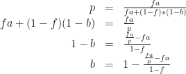
So, sticking with the parameters of our initial example (0.1% probability of service failure, 99% sensitivity) and deciding that we want a positive predictive value of at least 90% (so that 9 out of 10 alerts will mean something’s actually broken), we end up with

The necessary specificity is about 99.99% — that’s way higher than the sensitivity of 99%! In order to get a probe that detects failures in this service with sufficient reliability, you need to be 100 times less likely to falsely detect a failure than you are to miss a positive!
So listen.
You’ll often be tempted to favor high sensitivity at the cost of specificity, and sometimes that’s the right choice. Just be careful: avoid the base rate fallacy by remembering that your false-positive rate needs to be much smaller than your failure rate if you want your test to have a decent positive predictive value.
