Monitorama PDX was a fantastic conference. Lots of engineers, lots of diversity, not a lot of bullshit. Jason Dixon and his minions are some top-notch conference-runners.

As someone who loves to see math everywhere, I was absolutely psyched at the mathiness of the talks at Monitorama 2014. I mean, damn. Here, watch my favorite talk: Noah Kantrowitz’s.

I studied physics in college, and I worked in computational research, so the Fourier Transform was a huge deal for me. In his talk, Noah gives some really interesting takes on the application of digital signal processing techniques to ops. I came home inspired by this talk and immediately started trying my hand at this stuff.

What Fourier analysis is

“FOUR-ee-ay” or if you want to be French about it “FOO-ree-ay” with a hint of phlegm on the “r”.

Fourier analysis is used in all sorts of fields that study waves. I learned about it when I was studying physics in college, but it’s most notably popular in digital signal processing.

It’s a thing you can do to waves. Let’s take sound waves, for instance. When you digitize a sound wave, you _sample_ it at a certain frequency: some number of times every second, you write down the strength of the wave. For sound, this sampling frequency is usually 44100 Hz (44,100 times a second).

Why 44100 Hz? Well, the highest pitch that can be heard by the human ear is around 20000 Hz, and you can only reconstitute frequencies from a digital signal at up to half the sampling rate. We don’t need to capture frequencies we can’t hear, so we don’t need to sample any faster than twice our top hearing frequency.

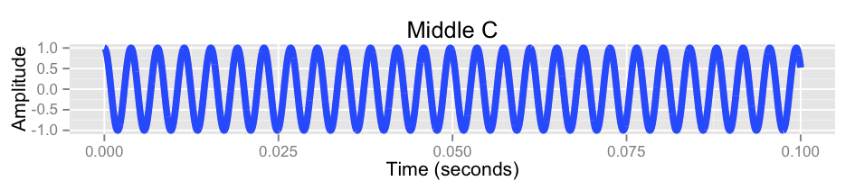
Now what Fourier analysis lets you do is look at a given wave and determine the frequencies that were superimposed to create it. Take the example of a pure middle C (this is R code):

library(ggplot2)
signal = data.frame(t=seq(0, .1, 1/44100))
signal$a = cos(signal$t * 261.625)
qplot(data=signal, t, a, geom='line', color=I('blue'), size=I(2)) +
    ylab('Amplitude') + xlab('Time (seconds)') + ggtitle('Middle C')

Pass this through a Fourier transform and you get:

fourier = data.frame(v=fft(signal$a))
# The first value of fourier$v will be a (zero) DC
# component we don't care about:
fourier = tail(fourier, nrow(fourier) - 1)
# Also, a Fourier transform contains imaginary values, which
# I'm going to ignore for the sake of this example:
fourier$v = Re(fourier$v)
# These are the frequencies represented by each value in the
# Fourier transform:
fourier$f = seq(10, 44100, 10)
# And anything over half our sampling frequency is gonna be
# garbage:
fourier = subset(fourier, f <= 22050)

qplot(data=fourier, f, v, geom='line', color=I('red'), size=I(2)) +
    ylab('Fourier Transform') + xlab('Frequency (Hz)') +
    ggtitle('Middle C Fourier Transform') + coord_cartesian(xlim=c(0,400))

As you can see, there’s a spike at 261.625 Hz, which is the frequency of middle C. Why does it gradually go up, and then go negative and asymptotically come back to 0? That has to do with windowing, but let’s not worry about it. It’s an artifact of this being a numerical approximation of a Fourier Transform, rather than an analytical solution.

You can do Fourier analysis with equal success on a composition of frequencies, like a chord. Here’s a C7 chord, which consists of four notes:

signal$a = cos(signal$t * 261.625 * 2 * pi) + # C
    cos(signal$t * 329.63 * 2 * pi) + # E
    cos(signal$t * 392.00 * 2 * pi) + # G
    cos(signal$t * 466.16 * 2 * pi) + # B flat
qplot(data=signal, t, a, geom='line', color=I('blue'), size=I(2)) +
    ylab('Amplitude') + xlab('Time (seconds)') + ggtitle('C7 chord')

Looking at that mess, you probably wouldn’t guess that it was a C7 chord. You probably wouldn’t even guess that it’s composed of exactly four pure tones. But Fourier analysis makes this very clear:

fourier = data.frame(v=fft(signal$a))
fourier = tail(fourier, nrow(fourier) - 1)
fourier$v = Re(fourier$v)
fourier$f = seq(10, 44100, 10)
fourier = subset(fourier, f <= 22050)

qplot(data=fourier, f, v, geom='line', color=I('red'), size=I(2)) +
    ylab('Fourier Transform') +
    xlab('Frequency (Hz)') +
    ggtitle('Middle C Fourier Transform') +
    coord_cartesian(xlim=c(0,400))

And there are our four peaks, right at the frequencies of the four notes in a C7 chord!

Straight-up Fourier analysis on server metrics

Naturally, when I heard all these Monitorama speakers mention Fourier transforms, I got super psyched. It’s an extremely versatile technique, and I was sure that I was about to get some amazing results.

It’s been kinda disappointing.

By default, a Graphite server samples your metrics (in a manner of speaking) once every 10 seconds. That’s a sampling frequency of 0.1 Hz. So we have a Nyquist Frequency (the maximum frequency at which we can resolve signals with a Fourier transform) of half that: 0.005 Hz.

So, if our goal is to look at a Fourier transform and see important information jump out at us, we have to be looking for oscillations that occur three times a minute or less. I don’t know about you, but I find that outages and performance anomalies rarely show up as oscillations like that. And when they do, you’re going to notice them before you do a Fourier transform.

Usually we get spikes or step functions instead, which bleed into wide ranges of nearby frequencies and end up being much clearer in amplitude-space than in Fourier space. Take this example of some shit hitting some fans:

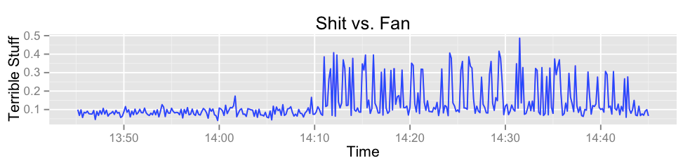
If we were trying to get information from this metric with Fourier transforms, we’d be interested in the Fourier transform before and after the fan got shitty. But those transforms are much less useful than the amplitude-space data:

I haven’t been able to find the value in automatically applying Fourier transforms to server metrics. It’s a good technique for finding oscillating components of a messy signal, but unless you know that that’s what you’re looking for, I don’t think you’ll get much else out of them.

What about low-pass filters?

A low-pass filter uses a Fourier transform to remove high frequency components from a signal. One of my favorite takeaways from that Noah Kantrowitz talk was this: Nagios’s flapping detection mechanism is a low-pass filter.

If you want to alert when a threshold is exceeded — but not every time your metric goes above and below that threshold in a short period of time — you can run your metric through a low-pass filter. The high-frequency, less-valuable data will go away, and you’ll be left with a more stable signal to check against your threshold.

I haven’t tried this method of flap detection, but I suspect that the low-sampling-frequency problem would make it significantly less useful than one might hope. If you’ve seen Fourier analysis applied as a flap detection algorithm, I’d love to see it. I would eat my words, and they’d be delicious.

I hope I’m wrong

If somebody can show me a useful application of Fourier analysis to server monitoring, I will freak out with happiness. I love the concept. But until I see a concrete example of Fourier analysis doing something that couldn’t be done effectively with a much simpler algorithm, I’m skeptical.

Addendum

As Abe Stanway points out, Fourier analysis is a great tool to have in your modeling toolbox. It excels at finding seasonal (meaning periodic) oscillations in your data. Also, Abe and the Skyline team are working on adding seasonality detection to Skyline, which might use Fourier analysis to determine whether seasonal components should be used.

Theo Schlossnagle coyly suggests that Circonus uses Fourier analysis in a similar manner.