I want to point out a paradox you may not have noticed.

A team of software engineers or SREs invariably has more good ideas than time. We know this very well. Pick any system we own, and we’ll come up with a list of 10 things we could do to make it better. Off the top of our head.

On the other hand, when our team is confronted with the opportunity to purge some old features or enhancements out of the backlog, there’s resistance. We say, “we might get around to this some day,” or “this still needs to get done.”

These two beliefs, taken together, reveal a deep lack of team self-confidence.

If our team always has more good ideas than time, then we’re never going to implement all the good ideas in our backlog. If we add more people, we’ll just get more good ideas, and the backlog will just get more bloated.

Why are we reluctant to ruthlessly remove old tickets, then? We know that we’re constantly generating good ideas. In fact, the ideas we’re generating today are necessarily (on average) better than most of the ideas in the backlog:

1. We have more information about the system now then we used to, so our new ideas are more aligned with real-world facts, and
2. We have more experience as engineers now, so we have developed better intuition about what kind of interventions will create the most value.

Seen in this light, a hesitance to let go of old ideas is revealed as a symptom of a deep pathology. It means we don’t believe in our own creativity and agency. If we did, we would have easy answers to the questions we always ask when we consider closing old tickets:

• What if we forget about this idea? That’s okay. We’ll have plenty of other, better, more relevant ideas. We never stop generating them.
• What if this problem gets worse over time? If the risk is enough that we should prioritize this ticket over our other work, then let’s do that now. Otherwise, we can cross that bridge if we ever get to it.
• Will the reporter of this ticket even let us close it? Nobody owns our backlog but us. When we decide to close a ticket, all we owe the reporter is an honest explanation of why.

Leave behind the paradox of the bloated backlog and start believing in your team’s own agency and creativity. Hell, maybe even cap your backlog. A team with faith in its competence is a team unleashed.

It’s good to have accurate and thorough metrics for our systems. But that’s only where observability starts. In order to get value out of metrics, we have to focus on the right ones: the ones that tell us about outcomes that matter to our users.

In The Latency/Throughput Tradeoff, we talked about why a given cluster can’t be optimized for low latency and high throughput at the same time. In conclusion, we decided that separate clusters should be provisioned for latency-centric use cases and throughput-centric use cases. And since these different clusters are optimized to provide different outcomes, we’ll need to interpret their metrics in accordingly different ways.

Let’s consider an imaginary graph dashboard for each type of cluster. We’ll walk through the relationships between metrics in each cluster, both under normal conditions and under excessive load. And then we’ll wrap up with some ideas about evaluating the capacity of each cluster over the longer term.

Metrics for comparison

In order to contrast our two types of clusters, we’ll need some common metrics. I like to employ the USE metrics at the top of my graph dashboards (more on that in a future post). So let’s use those:

• Utilization: The total CPU usage for all hosts in the cluster.
• Saturation: The number of queued requests.
• Error rate: The rate at which lines are being added to hosts’ error logs across the cluster.

In addition to these three metrics, we want to see a fourth metric. For the latency-optimized cluster, we want to see latency. And for the throughput-optimized cluster, we want to see throughput.

One of the best things about splitting out latency-optimized and throughput-optimized clusters is that the relationships between metrics become much clearer. It’s hard to tell when something’s wrong if you’re not sure what kind of work your cluster is supposed to be doing at any given moment. But separation of concerns allows us to develop intuition about our systems’ behavior and stop groping around in the dark.

Latency-optimized cluster

Let’s look at the relationships between these four important metrics in a latency-optimized cluster under normal, healthy conditions:

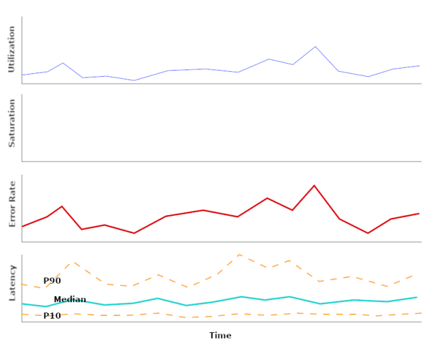Utilization will vary over time depending on how many requests are in flight. Saturation, however, should stay at zero. Any time a request is queued, we take a latency hit.\

Error rate would ideally be zero, but come on. We should expect it to be correlated to utilization, following the mental model that all requests carry the same probability of throwing an error.

Latency, then – the metric this cluster is optimized for – should be constant. It should not be affected by utilization. If latency is correlated to utilization, then that’s a bug. There will always be some wiggle in the long tail (the high percentiles), but for a large enough workload, the median and the 10th percentile should pretty much stay put.

Now let’s see what happens when the cluster is overloaded:

We start to see plateaus in utilization, or at least wider, flatter peaks. This means that the system is low on “slack”: the idle resources that it should always have available to serve new requests. When all resources are busy, saturation rises above zero.

Error rate may still be correlated with utilization, or it may start to do wacky things. That depends on the specifics of our application. In a latency-optimized cluster, saturation is always pathological, so it shouldn’t be surprising to see error rates climb or spike when saturation rises above zero.

Finally, we start to see consistent upward trends in latency. The higher percentiles are affected first and most dramatically. Then, as saturation rises even higher, we can see the median rise too.

Throughput-optimized cluster

The behavior of our throughput-optimized cluster, on the other hand, is pretty different. When it’s healthy, it looks like this:

Utilization – which, remember, we’re measuring via CPU usage – is no longer a fluffy cloud. Instead, it’s a series of trapezoids. When no job is in progress, utilization is at zero. When a job starts, utilization climbs up to 100% (or as close to 100% as reality allows it to get), and then stays there until the job is almost done. Eventually, the number of active tasks drops below the number of available processors, and utilization trails off back to zero.

Saturation (the number of queued tasks) follows more of a sawtooth pattern. A client puts a ton of jobs into the system, bringing utilization up to its plateau, and then as we grind through jobs, we see saturation slowly decline. When saturation reaches zero, utilization starts to drop.

Unlike that of a latency-optimized cluster, the error rate in a throughput-optimized cluster shouldn’t be sensitive to saturation. Nonzero saturation is an expected and desired condition here. Error rate is, however, expected to be follow utilization. If it bumps around at all, it should plateau, not sawtooth.

And finally, in the spot where the other cluster’s dashboard had a latency graph, we now have throughput. This we should measure in requests per second per job queued! What our customers really care about is not how many requests per second our cluster is processing, but how many of their requests per second. We’ll see why this matters so much in a bit, when we talk about this cluster’s behavior under excessive load.

Throughput should be tightly correlated to utilization and nothing else. If it also seems to exhibit a negative correlation to saturation, then that’s worth looking into: it could mean that queue management is inappropriately coupled to job processing.

Now what if our throughput-optimized cluster starts to get too loaded? What does that look like?

Utilization by itself doesn’t tell us anything about the cluster’s health. Qualitatively, it looks just like before: big wide trapezoids. Sure, there a bit wider than they were before, but we probably won’t notice that – especially since it’s only on average that they’re wider.

Saturation is where we really start to see the cracks. Instead of the sawtooth pattern we had before, we start to get more sawteeth-upon-sawteeth. These are jobs starting up on top of jobs that are already running. A few of these are to be expected even under healthy circumstances, but if they become more frequent, it’s an indication that there may be too much work for the cluster to handle without violating throughput SLOs.

Error rate may not budge much in the face of higher load. After all, this cluster is supposed to hold on to big queues of requests. As far as it’s concerned, nothing is wrong with that.

And that’s why we need to measure throughput in requests per second per job queued. If all we looked at was requests per second, everything would look hunky dory. But when there are two jobs queued and they’re constrained to use the same pool of processors, somebody’s throughput is going to suffer. On this throughput graph, we can see that happen right before our eyes.

Longer-term metrics

Already, we’ve seen how decoupling these two clusters gives us a much clearer mental model of their expected behavior. As we get used to the relationships between the metrics we’ve surfaced, we’ll start to build intuition. That’s huge.

But we don’t have to stop there! Having a theory (which is what we built above) also allows us to reason about long-term changes in the observable properties of these clusters as their workloads shift.

Take the throughput-optimized cluster, for instance. As our customers place more and more demand on it, we expect to see more sawteeth-upon sawtooth and longer intervals between periods of zero saturation. This latter observation is key, since wait times grow asymptotically as utilization approaches 100%. So, if we’re going to want to do evaluate the capacity needs of our throughput-optimized cluster, we should start producing these metrics on day one and put them on a dashboard:

• Number of jobs started when another job was already running, aggregated by day. This is the “sawteeth-upon-sawteeth” number.
• Proportion of time spent with zero saturation, aggregated by day.
• Median (or 90th percentile) time-to-first-execution for jobs, aggregated by day. By this I mean: for each customer job, how much time passed between the first request being enqueued and the first request starting to be processed. This, especially compared with the previous metric, will show us how much our system is allowing jobs to interfere with one another.

An analogous thought process will yield useful capacity evaluation metrics for the latency-optimized cluster.

TL;DR

Separating latency- and throughput-optimized workloads doesn’t just make it easier to optimize each. It carries the added benefit of making it easier to develop a theory about our system’s behavior. And when you have a theory that’s consistent with the signal and a signal that’s interpretable within your theory, you have observability.